THE SPECTROHELIOSCOPE
A spectrohelioscope is an instrument that enables the safe visual
observation of the Sun in monochromatic light across the visual
spectrum. It is basically a high dispersion spectroscope attached to
the focal plane of a telescope.
The spectroscope is used as a monochromator to isolate certain specific
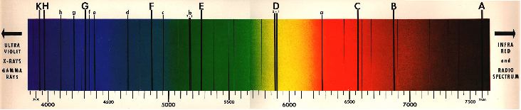
Solar Lines, notably the Fraunhofer C, D3, b3 & b4, F, H & K
absorption lines. The Solar image formed by the telescope is focused on
the entrance slit of the monochromator. In a Czerny-Turner
monochromator, the beam passing through the entrance slit is collimated
by a long focus spherical mirror and the parallel beam reflected at a
slight angle onto a plane diffraction grating which disperses the white
light into a long spectrum. The part of the spectrum of interest is
directed onto a second collimator which de-collimates the parallel beam
and focuses it onto an exit slit, normally co-planar to, and adjacent
to, the entrance slit. The wavelength at the exit slit is adjusted by
altering the tilt of the grating in the plane of the slits. The exit
slit is narrowed until only the core of the particular Fraunhofer
absorption line is contained within it.
The monochromatic image on the exit slit is then magnified using either
a long focus eyepiece, or re-imaged with a relay lens system. Because
the image at the exit slit is a thin line, it is ostensibly one
dimensional. To obtain a 2D image, the Solar image on the entrance
slit, and its corresponding counterpart focused onto the exit slit,
must be scanned synchronously. When the scan frequency is 24Hz or
faster, the eye sees a flicker free 2D image.
CZERNY-TURNER SHS - Chris Westland
To apply this principle to a practical instrument the monochromator
must have a spectral resolution of at least 11000 at the C line. This
places some physical constraints on the monochromator.
The minimum passband needed to detect faint Chromospheric detail in the
C line is Å0.6. The minimum useable slit width is about 10 microns.
Narrow slits are hard to use because they reduce image illumination and
introduce defects due to Fraunhofer diffraction, and longitudinal black
lines running the length of the spectrum caused by dust on the slit.
The minimum linear dispersion required is therefore Å0.6 in 10 microns,
which corresponds to Å60/mm. Because the slits have to be so narrow at
this working limit, for the illumination of the C line at the exit slit
to be sufficient for a useable scan width, the focal ratio of the
telescope would have to be about f/20. This is a relatively fast system
for an SHS, causing heating problems at the entrance slit.
Higher linear dispersion permits a narrower passband for a given slit
width. The ideal slit width is between 100 and 250 microns, and the
corresponding linear dispersion between Å6/mm & Å2.4/mm.
There are three ways to increase linear dispersion of the monochromator:
(i) increase the ruling density of the grating
(ii) increase the collimator focal length
(iii) use higher dispersion orders
A 600 groove/mm grating has orders 1 up to 8 in the violet.
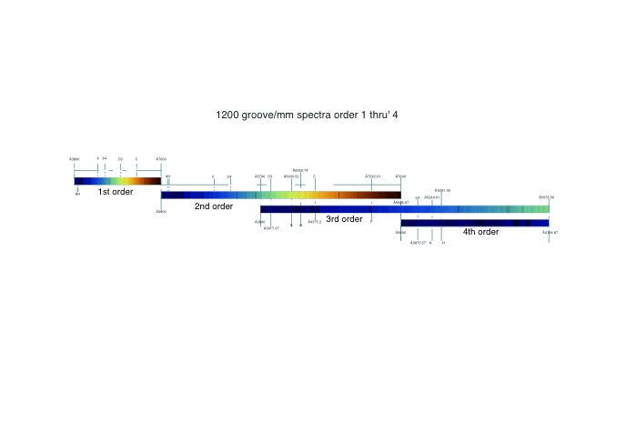
A 1200 groove/mm grating has orders 1 up to 4 in the violet.
A 1800 groove/mm grating has order 1 & up to green in order 2.
A 1800 groove/mm grating has a complete 1st order and 2nd order up to Å5555.56. There is no overlap between orders.
A 1200 groove/mm grating used in the 1st & 2nd order is optimum,
the grating is tilted too far over in the 3rd order and presents such a
reduced width that the image becomes too faint.
Observations with a 600 groove/mm grating are much more complicated
because of the overlapping orders. The grating may be used effectively
in the orders 1 thru' 3. Orders 4 & 5 are feasible, but very
problematic. The tilt of the grating is too great in orders 6 thru' 8.
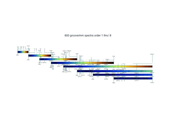
600 groove/mm grating:
1st Order:
K Å3933.68 passband Å10
H Å3968.49 passband Å9
F Å4861.34 passband Å0.4
b4 Å5167.33 passband Å0.2
D3 Å5875.6 passband Å0.1
C Å6562.82 passband Å0.5
2nd Order:
K Å3933.68 passband Å10
H Å3968.49 passband Å9
F Å4861.34 passband Å0.4
b4 Å5167.33 passband Å0.2
D3 Å5875.6 passband Å0.1 overlaps at Å3917.07 in the 3rd order - no filter needed
C Å6562.82 passband Å0.5 overlaps at Å4375.2 in the 3rd order - use Schott OG590
3rd Order:
K Å3933.68 passband Å10 overlaps at Å5900.52 in the 2nd order - use Schott BG3
H Å3968.49 passband Å9 overlaps at Å5952.74 in the 2nd order - use Schott BG3
F Å4861.34 passband Å0.4 overlaps at Å7292.01 in the 2nd order - use Schott RG695
b4 Å5167.33 passband Å0.2 overlaps at Å3875.57 in the 4th order - no filter needed
D3 Å5875.6 passband Å0.1 overlaps at Å3917.07 in the 3rd order - no filter needed
C Å6562.82 passband Å0.5 overlaps at Å4375.2 in the 3rd order - use Schott OG590
overlaps at Å3937.69 in the 4th order - no filter needed
4th Order:
K Å3933.68 passband Å10 overlaps at Å5244.91 in the 3rd order - use Schott BG3
H Å3968.49 passband Å9 overlaps at Å5291.32 in the 3rd order - use Schott BG3
F Å4861.34 passband Å0.4 overlaps at Å6481.79 in the 3rd order - use Schott RG695
b4 Å5167.33 passband Å0.2 overlaps at Å6889.89 in the 3rd order - use Schott RG715
overlaps at Å4133.94 in the 5th order
D3 Å5875.6 passband Å0.1 overlaps at Å4700.48 in the 5th order - use Schott GG495
overlaps at Å3917.07 in the 6th order
C Å6562.82 passband Å0.5 overlaps at Å5250.26 in the 5th order - use Schott OG590
overlaps at Å4375.21 in the 7th order
5th Order:
K Å3933.68 passband Å10 overlaps at Å4917.1 in the 4th order - use Schott BG3
overlaps at Å6556.13 in the 3rd order
H Å3968.49 passband Å9 overlaps at Å4960.61 in the 4th order - use Schott BG3
overlaps at Å6614.15 in the 3rd order
F Å4861.34 passband Å0.4 overlaps at Å6076.68 in the 4th order - use Schott BG23
overlaps at Å4051.12 in the 6th order
b4 Å5167.33 passband Å0.2 overlaps at Å6459.28 in the 4th order - use Schott BG39
overlaps at Å4133.94 in the 5th order
D3 Å5875.6 passband Å0.1 overlaps at Å7344.5 in the 4th order - use Schott GG420
overlaps at Å4896.33 in the 6th order
overlaps at Å4196.86 in the 7th order
C Å6562.82 passband Å0.5 overlaps at Å5469.02 in the 6th order - use Schott OG570
overlaps at Å4687.73 in the 7th order
overlaps at Å4101.76 in the 8th order
The ideal working focal ratio for the monochromator to obtain a
comfortable image brightness is between f/25 & f/45. Focal ratios
greater than f/45 result in a very dim image except at restricted scan
widths.
The heart of the monochromator is the plane diffraction grating. They
are supplied as either ruled or holographic replicas. The grating
should preferably be a ruled replica with a quantum efficiency between
60% & 80% at the desired blaze wavelength, and a theoretical
resolution of between 80% & 90%. That is there should only be
between 10% & 20% defects on the replica compared to its master.
The glass substrate should also be not less than 10mm thick. Plane
gratings are normally either square or rectangular.
The higher the ruling density, the finer the spectral resolution for a
given ruled width. Observations are normally made in the first order in
the C line and either 1st or 2nd order in the K line. The second order
spectrum has approximately three times the angular dispersion of the
first order.
Ruling densities vary from 600 groove/mm to 3200 groove/mm. Large
gratings with high ruling densities tend to be holographic only because
it is not practicable to mechanically rule the master. Holographic
gratings are more accurate in terms of uniformity of groove spacing and
groove defects, but they typically have a slightly lower quantum
efficiency.
Throughout most of the C20th gratings were only available with either
600 groove/mm or 1200 groove/mm ruling densities. In the case of a 600
groove/mm grating the 1st & 2nd orders do not overlap, but the 2nd
and 3rd orders overlap. To observe the K line in the 3rd order a blue
filter needs to be placed in front of the exit slit to block light from
the green part of the 2nd order spectrum. In the case of a 1200
groove/mm grating the 1st & 2nd orders do not overlap, but there is
overlap between the violet end of the 3rd order spectrum and the orange
and red end of the 2nd order spectrum. However the violet end of the
3rd order spectrum is so faint visually compared to the yellow and
orange of the 2nd order that observation in the He D3 line is possible
without a minus violet filter. Observation in the C-line in the 2nd
order is possible with a red narrow-cut filter. A 1800 groove/mm
grating produces a 1st order spectrum and a 2nd order spectrum that
does not overlap, but the 2nd order only runs from the violet to the
green, by which time the grating is tilted in excess of 80º. It is
possible to observe in the K-line in the 2nd order without using a blue
filter.
In the first half of the C20th, the highest ruling density was 600
groove/mm or a close imperial equivalent (15,000 grooves per inch).
There was no reliable replication process either. All plane gratings
were ruled masters, having grooves cut mechanically with a diamond, the
ruling machine being an interferometer controlled dividing engine.
Gratings were ruled on speculum metal, which even when freshly polished
had only 65% transmission efficiency. Gratings needed to be much larger
due to their lower ruling density, and consequently their cost was
prohibitive. The speculum metal also inevitably tarnished, and it was
not possible to effectively remove the oxidation.
During the latter half of the C20th it became possible to rule a master
grating on a thick evaporated metallic film deposited on the substrate
in a vacuum tank. Replicas were made of the master by placing a layer
of epoxy resin against its ruled surface, waiting for it to cure, and
then carefully separating them. The replica could then be aluminised.
Replicas with 90% accuracy to their master are now comparatively
affordable. They are also far more durable.
Light may be concentrated into a desired portion of the spectrum by a
process known as "blazing". The ruled groove profile is intentionally
inclined at what is termed the "blaze angle". For visual use across the
spectrum from Å3800 to Å7000, the optimum blaze wavelength is Å5000.
The quantum efficiency of the grating is greatest at the blaze
wavelength. For use in an SHS it needs to be higher than 60% and
preferably 80% at the blaze wavelength. The blaze wavelength and
quantum efficiency changes with the spectral order. A blaze wavelength
of Å5000 in the 1st order becomes Å2500 in the 2nd order. A QE of 80%
at the blaze wavelength in the 1st order becomes 40% in the 2nd order,
and so on.
To build a SHS with a resolution comparable to the very best
Fabry-Perot etalon notch filters, a grating ruled at either 1200
groove/mm or 1800 groove/mm, blazed at Å5000, with a QE > 80% must
be used in a monochromator with a linear dispersion not less than 6Å/mm.
THE IMAGE SYNTHESISER
Before proceeding further into the design of the monochromator, there
is the consideration of the synthesiser which scans the 1D image and
converts it into a 2D image. There have been several ways devised to do
this, and they fall into two categories; scanners that scan the
monochromator slits across the image, and scanners that scan the image
across fixed slits.
The first SHS was designed and built by George Ellery Hale in the mid
1920's. Hale's SHS scanned the slits over the image. The slits were
carried by a light bar that oscillated about a central pivot. He also
tried two other arrangements, sideways oscillating slits, and a
rotating glass disc cut with many radial slits. The rotating glass disc
was invented for use in a Spectroheliograph by F. Stanley in 1912. Hale
and Mitchell fitted one to the spectrograph of the Mt. Wilson 60 foot
Solar Tower telescope in 1929. Hitchcock, a Mt. Wilson technician cut
an 8-inch glass disk with first of all 50, and later 150 slits. Veio
developed this form of scanner further in the mid 1960's, employing 24
slits. There are two other moving slit scanners, the reciprocating
oscillating slit scanner developed by F.J. Seller's in the late 1920's
and the reciprocating rod with slits invented by B.G. Manning in 1979.
The alternative to scanning the slits over the image is to scan the
image across the slits. This was first done by J.A. Anderson in 1929.
Anderson placed narrow dense flint cubical prisms in front of both
slits, and scanned a small width of the complete image by rotating them
about their longitudinal axes. Eddison Petit used a similar arrangement
but with separately mounted prisms and motors. The Spacek Co. tried a
single long cubical prism mounted in a central bearing.
A different technique involves the use of nodding mirrors. This was
first suggested by Sinclair Smith in 1929. It was first realised by
Jeffery Young in the early 1970's. It was subsequently perfected by
Vittorio Lovato, Italy; Toshio Ohnishi, Japan; and Leonard Higgins
& Fred Veio, California. Fred Veio turned the surname initial
letters into the acronym HYLOV. The HYLOV synthesiser consists
essentially of a pair of mirrors carried on a spindle supported by
bearings at either end. The mirrors are nodded to and fro with a
frequency of 15Hz.
Another nodding mirror synthesiser was developed quite recently (2002)
by Camiel Severijns, (Netherlands). It comprises a pair of separately
driven mirrors, one in front of each slit, oscillating at 12Hz in
anti-phase.
A nodding mirror synthesiser as yet untried was suggested by George Y.
Haig in 1998. It comprises a single double sided mirror, placed in a
folded light path equidistant between the entrance and exit slits.
The advantage of scanning the slits across the image is that the beam
illuminating the collimators and grating remains parallel to the chief
ray. It is simpler to size the monochromator and telescope optics to
minimize vignetting.
The disadvantages of moving slit scanners are that they become a source
of vibration which must be damped, and it is almost impossible to
adjust the slit width and hence the passband whilst the scanner is
running.
Anderson, Petit and Spacek prisms offer a way around the limitations of
moving slit scanners without tilting the light path, as occurs in the
HYLOV, Severijns and Haig synthesisers. The difficulty with cubical
prisms is their inherently restricted scan height, unless the face
width is 1.5 times the Solar image diameter. The scan amplitude is also
fixed. The only way to vary the brightness of the scanned image is to
either alter the slit width, which affects contrast and resolution, or
vary the scan speed. There is a limit to how low the scan speed can be,
typically about 5 revs/ sec, corresponding to a 20Hz scan rate.
All nodding mirror synthesisers tilt the light path causing it to move
back and forth across the collimators. A less obvious consequence is
the concomitant tilt of the aperture stop (the grating) across the
telescope objective. Both telescope objective and collimators must be
sized to accommodate the lateral movement of the light path if
vignetting is to be avoided at the scan limit. The scan height can be
varied by altering the oscillation amplitude.
Anderson, Petit and Spacek prisms do not tilt the light path.
Refraction through the tilted prism face deviates the light path whilst
maintaining parallelism to the chief ray.
The maximum useful scan height is 2000 arcsecs. The higher the scan
height the fainter the image becomes. To obtain an acceptable image
brightness at a 2000 arcsec scan height there must be sufficient light
in the C line in the exit slit. That is why the monochromator focal
ratio must be between f/20 and f/40.
DESIGNING MY CZERNY-TURNER SHS
After discussing the generalities of SHS design with Fred Veio, and
quizzing Camiel Severijns about his relatively compact SHS, I decided
to go for a full blown SHS capable of scanning a 31mm Solar image. I
already had a pair of 10-inch f/12.8 paraboloidal primaries in Duran 50
made some time ago by Jim Hysom of Hytel Optics. Despite having 2-inch
perforations (they had been intended for a Nasmyth-Cassegrain optic set
for the Calver - which I subsequently abandoned), I felt they would
serve well for the Czerny-Turner collimators. To obtain a 31mm image
size I selected a 6-inch f/21 Littrow doublet from D&G Optical, and
to obtain the necessary spectral resolution a Diffraction Products
110mm x 110mm x16mm, 1200 groove/mm ruled 100mm x 100mm replica grating
blazed for Å5461, QE 80%, theoretical resolution 90%.
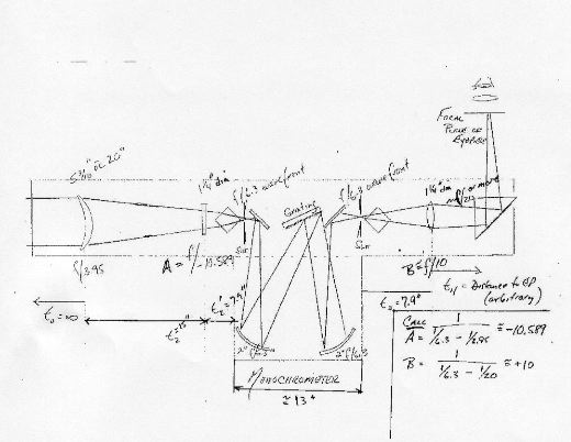
The grating ruling diagonal is 141mm or 5.55-inches. The collimators
are 128-inch focal length, so the f/ratio of the telescope needed to be
128/5.55 = 23. I decided to use Anderson prisms mounted vertically in
front of vertical slits, all in the same plane as the collimators and
grating. The edge of each collimator mirror would be used, a 7.2-inch
square aperture. The axes of the parabolic mirrors would be directed to
the optical axis of the grating, reducing spherical aberration, coma
and astigmatism at the exit slit, in the 1st order, to zero.
It is possible to have the slits and the collimators both in the
horizontal plane, and to skew the grating towards the second
collimator. The grating rulings also need to be horizontal. As the
grating is tilted a vertical spectrum is thrown onto the second
collimator. Although this arrangement makes for a mechanically simpler
prism drive, skewing the grating (by half the deviation angle) tilts
the spectral lines on the exit slit. In my case it would have been a
2º.82 tilt, which across a 31mm long slit amounts to 1.53mm. Horizontal
slits and collimators are only workable with long focal ratio mirrors
and short slit lengths and restricted scan amplitudes.
Because the three mirror Czerny-Turner monochromator reverts the image,
the Anderson prisms would be contra-rotated to synthesise a coherent
image. Both prisms would be driven by a single variable speed DC motor
through a T-bevel reversing gearbox, OnDrive BLHM30-1, and a pair of
T-bevel gearboxes, OnDrive BLHT30-1. The DC motor would be controlled
by a chopper cct. and varied between 300 rpm and 600 rpm. The prisms
would be mounted in cylindrical cells held in cage bearings, and
supported at each end to prevent wobbling.
The spectral resolution (90%) at the C line is Å0.060, good even for
passbands down to Å0.1, used on the Magnesium b3 & b4 lines in the
2nd order. The grating's angular dispersion was 23º.2 and the 1st order
linear dispersion Å2.356/mm, giving a spectrum length between Å3800
& Å7600 of 1583.6mm or 5ft. 2".3. For a Å0.6 passband in the C-line
the slit width would need to be 250 microns or 10 thou. More than
adequate. A 100 micron (4 thou) slit width would give a passband of
Å0.24. There would be sufficient light even with a 100 micron slit to
scan the 31mm image height and provide a contrasty image with a visual
brightness comparable to a bright Total Lunar Eclipse.
Vignetting at the square grating amounts to 33% due to the paraxial
rays fully illuminating its diagonal. Vignetting at the collimators is
6% due to their being used off axis. Light loss at the collimators due
to the 2-inch central perforation is 7%. Total system vignetting is
39%. There is no additional vignetting at the scan limit, the image is
uniformly illuminated. The reason the collimators are used off axis is
to keep the slit separation down to 12-inches and the deviation angle
as small as physically possible. The greater the deviation angle the
greater the astigmatism and coma at the image plane.
Used in the 2nd order the linear dispersion increases to Å0.788/mm
giving a spectrum length between Å3800 & Å7600 of 4388.2mm or 14ft.
4".8. For a Å0.5 passband in the C-line the slit width would need to be
600 microns or 24thou. Even with the reduced QE (40%), the image would
be slightly brighter.
Observations could be made at the following wavelengths:
1st Order:
K Å3933.68 passband Å10 slit width 4000 microns
H Å3968.49 passband Å9 slit width 3655 microns
F Å4861.34 passband Å0.4 slit width 160 microns
b4 Å5167.33 passband Å0.2 slit width 80 microns
D3 Å5875.6 passband Å0.1 slit width 40 microns
C Å6562.82 passband Å0.5 slit width 210 microns
2nd Order:
K Å3933.68 passband Å10 slit width 8850 microns
H Å3968.49 passband Å9 slit width 7985 microns
F Å4861.34 passband Å0.4 slit width 380 microns
b4 Å5167.33 passband Å0.2 slit width 200 microns
D3 Å5875.6 passband Å0.1 slit width 110 microns overlaps at Å3917.07 in the 3rd order - no filter needed
C Å6562.82 passband Å0.5 slit width 630 microns overlaps at Å4375.2 in the 3rd order - use Schott OG590
3rd Order:
K Å3933.68 passband Å10 slit width 16575 microns overlaps at Å5900.52 in the 2nd order - use Schott BG3
H Å3968.49 passband Å9 slit width 15050 microns overlaps at Å5952.74 in the 2nd order - use Schott BG3
F Å4861.34 passband Å0.4 slit width 970 microns overlaps at Å7292.01 in the 2nd order - use Schott RG695
b4 Å5167.33 passband Å0.2 slit width 635 microns overlaps at Å3875.57 in the 4th order - no filter needed
4th Order:
K Å3933.68 passband Å10 slit width 47360 microns overlaps at Å5244.91 in the 3rd order - use Schott BG3
H Å3968.49 passband Å9 slit width 40600 microns overlaps at Å5291.32 in the 3rd order - use Schott BG3
The telescope and monochromator I
decided would be laid out in an elevated timber building 20ft x 8ft,
total roof height 14ft, the floor 7ft above ground, giving 7ft working
height. The telescope would be fed by a 12-inch simple Heliostat
located at the entrance pupil 132.41-inches in front of the OG,
microstep driven in alt-az. The Heliostat in this location acts as the
entrance stop, preventing oblique rays entering the monochromator. I
ordered a 12-inch Duran 50 flat off Jim Hysom. I also decided to
microstep drive the grating using a stepper motor with an integral
planetary gearhead connected to a sine bar linkage. The stepper motor
controller's hand paddle would have an LCD display showing the
wavelength on the exit slit in Ångstroms.
I laid out the dimensions of the telescope's offset, and those of the
relay system so I could also observe the white light image using an
auxiliary eyepiece parallel to the relay lens system. A removable
diagonal mirror held in a kinematic mount could be placed in the light
path to the entrance slit. This would be a circular optical window
given a dielectric coating on the first surface. When removed the light
is transmitted onto the entrance slit. In this way it would be possible
to compare the white light and monochromatic images from the same
observing position. It would also be a simple matter to employ the
refractor for night time observations simply by deploying the optical
window. Infra-red radiation is absorbed by a Schott heat filter a short
distance in front of the Anderson prism. Martin Gautrey of Apex
re-polished the stock filter flat to ±1/10th wave.
The relay lens and re-imaging lens reduces the image diameter to 20.7mm
to comfortably accommodate it on a 35mm film format. There is also
another re-imaging lens which maintains the prime image diameter for
low power SHS work. Re-imaging the monochromatic image at the exit slit
enables the use of conventional eyepieces.

A low power telescope placed within the central perforation of the
second collimator mirror enables direct examination of the Solar
spectrum at a reduced spectral resolution. A similar auxiliary
telescope located within the central perforation of the first
collimator mirror provides a simultaneous white light view when the
scanner is running, albeit of the limb. Both these telescopes are
focused on the slits, and may also be used to enable accurate
collimation.
PARAXIAL MODEL OF SHS
• A heliostat mirror M1, F = É, D = 12 ins
• Entrance Stop S1, D = 6.21 ins
• An achromatic object glass OG1, F = 126 ins, D = 6 ins
• Heat filter F1, D = 1.97 ins
• Anderson prism P1, face width 1.815 ins
• Entrance Slit1 height 1.25 ins
• Collimator mirror Coll1, F = 128 ins, D = 10 ins
• Square reflection diffraction grating, G, L = 4.33 ins
• Collimator mirror Coll2, F = 128 ins, D = 10 ins
• Exit Slit2 height 1.25 ins
• Anderson prism P2, face width 1.815 ins
• Elliptical flat mirror M2, minor axis 3.25 ins
• Achromatic relay lens OG2, F = 35.433 ins, D = 3.15 ins
• Achromatic re-imaging lens OG3a, F = 35.433 ins, D = 3.15 ins
• Alternative re-imaging telephoto lens OG3b, F = 23.622 ins, D = 2.953 ins
• Eyepiece E1, Huyghenian, F = 4.75 ins, D = 2.125 ins
The Entrance Stop located 24 inches in front of the OG restricts the
angle of oblique rays to 1000 arcsecs. The Heliostat located at the
Entrance Pupil also restricts those oblique rays. The virtual image of
the Entrance Pupil formed by the first collimator mirror lies 2602.667
inches behind the grating, (1/2602.667 = 1/122 - 1/128). The Entrance
Pupil lies 132.41 inches in front of the objective, (1/132.41 = 1/126 -
1/2602.667). Because the monochromator section is symmetric, the Exit
Pupil lies 2602.667 inches behind the second collimator mirror. The
Petzval sum for the monochromator section, not including the relay and
re-imaging section is 42.442 inches (1/42.442 = 1/126 + 1/128 + 1/128).
The Petzval sum for the matched pair of relay and re-imaging lenses is
17.717 inches (1/17.717 = 1/35.433 + 1/35.433). The combined Petzval
sum is 12.499 inches (1/12.499 = 1/42.442 + 1/17.717). The sagittal
field curvature over the 1.2217 inch image diameter is 0.0149 inches.
Depth of focus for an f/21 effective focal ratio and 1/10th wavefront
(P - V) error is 0.0155 inches.
RAY HEIGHTS (Thin Component Ray Trace)
The Gaussian or 1st order model where the apertures are small compared
to separations and focal lengths is determined as follows:
System Data: d, the distance to the next component
K, the power of the current component = 1/focal length
Ray Tracing: h, the ray height at the current component
u' the angle between ray and axis leaving the current component (radians)
Sign conventions: h positive above axis, negative below
u' positive if ray descends in direction of travel
Calculations: u' after component = (previous) u' plus (current) h x K (i.e. u' = u + h x K)
h at following component = (previous) h minus (current) d x u' (i.e. h' = h - d x u')
The following results are for the principal rays both oblique and paraxial for a 2000 arcsec scan width
Oblique ray from below optical axis @ 1000 arcsecs
Component OG d = 126 K = 0.00793650794 h = -3 u' = -0.02865079365
Component Slit 1 d = 128 K = 0 h = 0.61 u' = -0.02865079365
Component Coll 1 d = 122 K = 0.0078125 h = 4.2773015873 u' = 0.004765625
Component Grating d = 122 K = 0 h = 3.6958953373 u' = 0.004765625
Component Coll 2 d = 128 K = 0.0078125 h = 3.1144890873 u' = 2.9097571e-2
Component Slit 2 d = 0 K = 0 h = -0.61 u' = 2.9097571e-2
Oblique ray from above optical axis @ 1000 arcsecs
Component OG d = 126 K = 0.00793650794 h = 3 u' = 0.01896825397
Component Slit 1 d = 128 K = 0 h = 0.61 u' = 0.01896825397
Component Coll 1 d = 122 K = 0.0078125 h = -1.817936508 u' = 0.004765625
Component Grating d = 122 K = 0 h = -2.399342758 u' = 0.004765625
Component Coll 2 d = 128 K = 0.0078125 h = -2.980749008 u' = 1.8521477e-2
Component Slit 2 d = 0 K = 0 h = -0.61 u' = 1.8521477e-2
Oblique ray from above optical axis @ 1000 arcsecs
Component OG d = 126 K = 0.00793650794 h = -3 u' = -0.02865079365
Component Slit 1 d = 128 K = 0 h = -0.61 u' = 0.02865079365
Component Coll 1 d = 122 K = 0.0078125 h = -4.2773015873 u' = -0.004765625
Component Grating d = 122 K = 0 h = -3.6958953373 u' = -0.004765625
Component Coll 2 d = 128 K = 0.0078125 h = -3.1144890873 u' = 2.9097571e-2
Component Slit 2 d = 0 K = 0 h = 0.61 u' = 2.9097571e-2
Oblique ray from below optical axis @ 1000 arcsecs
Component OG d = 126 K = 0.00793650794 h = -3 u' = -0.01896825397
Component Slit 1 d = 128 K = 0 h = -0.61 u' = -0.01896825397
Component Coll 1 d = 122 K = 0.0078125 h = 1.817936508 u' = -0.004765625
Component Grating d = 122 K = 0 h = 2.399342758 u' = -0.004765625
Component Coll 2 d = 128 K = 0.0078125 h = -2.980749008 u' = 1.8521477e-2
Component Slit 2 d = 0 K = 0 h = 0.61 u' = 1.8521477e-2
Paraxial ray from below optical axis
Component OG d = 126 K = 0.00793650794 h = -3 u' = -0.02380952381
Component Slit 1 d = 128 K = 0 h = 0 u' = -0.02380952381
Component Coll 1 d = 122 K = 0.0078125 h = 3.047619048 u' = 0
Component Grating d = 122 K = 0 h = 3.0476190476 u' = 0
Component Coll 2 d = 128 K = 0.0078125 h = 3.0476190476 u' = 2.3809524e-2
Component Slit 2 d = 0 K = 0 h = 0 u' = 2.3809524e-2
Paraxial ray from above optical axis
Component OG d = 126 K = 0.00793650794 h = 3 u' = 0.02380952381
Component Slit 1 d = 128 K = 0 h = 0 u' = 0.02380952381
Component Coll 1 d = 122 K = 0.0078125 h = -3.047619048 u' = 0
Component Grating d = 122 K = 0 h = -3.0476190476 u' = 0
Component Coll 2 d = 128 K = 0.0078125 h = -3.0476190476 u' = 2.3809524e-2
Component Slit 2 d = 0 K = 0 h = 0 u' = 2.3809524e-2

APERTURE STOP & FIELD LENS
Plotting these ray heights enables the location of the Aperture Stop to
be identified. The Aperture Stop is an element of an optical system
that determines the amount of light reaching the image. In a
monochromator ideally the Aperture Stop should be located at the
grating. In my design this would necessitate the separation of grating
and collimators be increased to 255 inches which would place it 127
inches in front of the slits, alongside the OG, in a mechanically
impractical position. Placing the grating 122 inches from the
collimators, 4 inches behind the slits, puts the Aperture Stop 134.64
inches after the grating, or 12.64 inches beyond the second collimator
mirror. This results in significant vignetting of the oblique rays at
the grating. The paraxial rays fully illuminate the grating. The
oblique rays entering the objective at an angle of 1000 arcsecs are
vignetted 56%. This results in the scanned image being half as bright
at the scan limit as at the scan centre.
To bring the Aperture Stop onto the grating a Field Lens is required,
either immediately in front of, or behind the entrance slit. The
purpose of the Field Lens is to redirect the oblique rays onto the
grating. The lens can be either bi-convex, plano-convex or positive
meniscus. Because the focal ratio of my objective is comparatively
fast, and because of problems that could arise through mutual
reflections off the Anderson prism, I decided to place the Field Lens
behind the entrance slit, located in the same cell as the adjustable
iris.
To determine the power of the Field Lens use the formula 1/fc= 1/u1 +
1/v, where fc is the focal length of the collimator, v1 the separation
of the grating and collimator and u1 the distance of the virtual image
of the Entrance Pupil formed by the first collimator mirror. Hence u =
-2602.667. To find the value of f for the Field Lens, we know that the
field lens conjugates are u2 = 126 and v2 = 128 + 2602.667 = 2730.667.
These values are then substituted into the formula 1/fl = 1/u2 + 1/v2,
which gives fl = 120.44 inches.
I had considerable difficulty trying to procure this component.
Eventually I found a suitable stock BK7 plano-convex lens in
OptoSigma's catalogue They could supply a 50mm x 3000mm focal length
plano-convex lens in crown glass broadband a/r coated on both sides.
The plane side faces the slit. Because the lens is near the focal plane
of the objective, and only a thin vertical section is illuminated, the
overall accuracy does not need to be better than 1/4 wave.
The following results are for the principal rays both oblique and
paraxial for a 2000 arcsec scan width with the field lens located 2
inches behind the entrance slit:
Oblique ray from below optical axis @ 1000 arcsecs
Component OG d = 126 K = 0.00793650794 h = -3 u' = -0.02865079365
Component Slit 1 d = 2 K = 0 h = 0.61 u' = -0.02865079365
Component FL 1 d = 126 K = 8.3028894e-3 h = 0.6673015873 u' = 2.3110262e-2
Component Coll 1 d = 122 K = 0.0078125 h = 3.5791946461 u' = 0.0048521958
Component Grating d = 122 K = 0 h = 2.9872267583 u' = 0.0048521958
Component Coll 2 d = 128 K = 0.0078125 h = 2.3952588706 u' = 2.3565156e-2
Component Slit 2 d = 0 K = 0 h = -6.2108106e-1 u' = 2.3565156e-2
Oblique ray from above optical axis @ 1000 arcsecs
Component OG d = 126 K = 0.00793650794 h = 3 u' = 0.01896825397
Component Slit 1 d = 2 K = 0 h = 0.61 u' = 0.01896825397
Component FL 1 d = 126 K = 8.3028894e-3 h = 5.7206349e-1
Component Coll 1 d = 122 K = 0.0078125 h = -2.416408776 u' = 4.8398403e-3
Component Grating d = 122 K = 0 h = -3.006869294 u' = 4.8398403e-3
Component Coll 2 d = 128 K = 0.0078125 h = -3.597329812 u' = 2.3264299e-2
Component Slit 2 d = 0 K = 0 h = -6.1949956e-1 u' = 2.3264299e-2e-2
Oblique ray from above optical axis @ 1000 arcsecs
Component OG d = 126 K = 0.00793650794 h = -3 u' = -0.02865079365
Component Slit 1 d = 2 K = 0 h = -0.61 u' = 0.02865079365
Component FL 1 d = 126 K = 8.3028894e-3 h = 5.7206349e-1 u' = 2.3718034e-2
Component Coll 1 d = 122 K = 0.0078125 h = 2.4164087763 u' = 4.8398403e-3
Component Grating d = 122 K = 0 h = 3.0068692942 u' = 4.8398403e-3
Component Coll 2 d = 128 K = 0.0078125 h = 3.5973298122 u' = 2.3264299e-2
Component Slit 2 d = 0 K = 0 h = 6.1949956e-1 u' = 2.3264299e-2
Oblique ray from below optical axis @ 1000 arcsecs
Component OG d = 126 K = 0.00793650794 h = -3 u' = -0.01896825397
Component Slit 1 d = 2 K = 0 h = -0.61 u' = -0.01896825397
Component FL 1 d = 126 K = 8.3028894e-3 h = 6.6730159e-1 u = 2.3110262e-2
Component Coll 1 d = 122 K = 0.0078125 h = -3.579194646 u' = 4.8521958e-3
Component Grating d = 122 K = 0 h = -2.987226758 u' = 4.8521958e-3
Component Coll 2 d = 128 K = 0.0078125 h = -2.395258871 u' = 2.3565156e-2
Component Slit 2 d = 0 K = 0 h = 6.2108106e-1 u' = 2.3565156e-2
Paraxial ray from below optical axis
Component OG d = 126 K = 0.00793650794 h = -3 u' = -0.02380952381
Component Slit 1 d = 2 K = 0 h = 0 u' = -0.02380952381
Component FL 1 d = 126 K = 8.3028894e-3 h = 4.7619048e-2 u = 2.3414148e-2
Component Coll 1 d = 122 K = 0.0078125 h = 2.9978017112 u' = 6.17775e-6
Component Grating d = 122 K = 0 h = 2.9970480263 u' = 6.17775e-6
Component Coll 2 d = 128 K = 0.0078125 h = 2.9962943414 u' = 2.3414727e-2
Component Slit 2 d = 0 K = 0 h = 7.9075137e-4 u' = 2.3414727e-2
Paraxial ray from above optical axis
Component OG d = 126 K = 0.00793650794 h = 3 u' = 0.02380952381
Component Slit 1 d = 2 K = 0 h = 0 u' = 0.02380952381
Component FL 1 d = 126 K = 8.3028894e-3 h = 4.7619048e-2 u = 2.3414148e-2
Component Coll 1 d = 122 K = 0.0078125 h = -2.997801711 u' = -6.17775e-6
Component Grating d = 122 K = 0 h = -2.997048026 u' = -6.17775e-6
Component Coll 2 d = 128 K = 0.0078125 h = -2.996294341 u' = 2.3414727e-2
Component Slit 2 d = 0 K = 0 h = 7.9075137e-4 u' = 2.3414727e-2
The aperture stop at the grating is 6.014 inches diameter. The grating
diagonal is 5.55 inches, so the vignetting is considerably reduced, and
the spectral resolution will be constant across the 2000 arcsec scan
width.
Adding a field lens modifies the Petzval Sum by an additional 1/f*n,
which for a 120.44-inch focus lens in BK7 is 1/120.44*1.5, decreasing
the field radius of curvature to 11.69 inches.

Optical Components List:
diffraction grating: 110mm x 110mm x16mm Pyrex, replica ruled 1200
groove/mm blaze wavelength Å5461 supplied by Diffraction Products Inc
cost $1458.55 (£791.27) inc shipping
Littrow object glass 6-inch f/21 1/20th wave MgF2 a/r coated @ Å5500,
with collimation cell, dust cap and custom OTA supplied by D & G
Optical cost $995 (£544.34) for the OG and $700 (£382.96) for the OTA
shipping extra
elliptical diagonal flat mirror: David Hinds 3.25-inch minor axis x
4.6-inch major axis x 15.88mm t Duran 50 fine annealed, 60-40 1/20th
wave @ Å6328, enhanced aluminium R>95% Å4500 - Å6500
plane parallel optical window: Perkin Elmer 90mm dia. x 21mm t fused
silica A 60-40 1/20 wave MgF2 a/r coated @ Å5500 both sides,
parallelism 5"arc cost $175 (£95.74) + shipping
heat filter - 1 off: Edmund Scientific T45-648 50mm dia. x 3mm t Schott
KG-1 60-40 scratch dig 1/10th wave, 92% IR reflectance factor, MgF2 a/r
coated @ Å5500 both sides, parallelism 1' arc cost £37.49 + VAT
line shifter - plane parallel optical window: PerkinElmer 50.5mm dia. x
15mm t BK7 grade A 60-40 1/20 wave MgF2 a/r coated @ Å5500 both sides,
parallelism 1'arc cost $48.50 (£26.53) + shipping
Anderson Prisms - 2 off: Apex cubical specials - 46mm x 35mm BK7 grade
A fine annealed 60-40 1/8th wave @ Å6328, 1'arc parallelism, 40 arcsec
max taper, with 40mm dia. x 10mm t BK7 cemented cylindrical end pieces.
35mm edges polished sharp, broadband a/r coated, cost £387.
Field Lens - 1 off: OptoSigma - 50mm x 3000mm Plano-Convex Crown Glass
20-10 1/4 wave broadband a/r coated @ Å4250 - Å6750 both sides, stock
no. 011-3390-A55 c/o LASER2000 £56.65 + £9.92 shipping
Relay lens: Surplus Shed achromatic doublet in cell 80mm dia. x 900mm fl a/r coated cost $29 (£15.87) + shipping
Re-imaging lens: Surplus Shed achromatic doublet in cell 80mm dia. x 900mm fl a/r coated cost $29 (£15.87) + shipping
Re-imaging lens: Andrews Cameras, Teddington, London second hand Tamron
300mm f/2.8 semi-apo with X2 converter Adaptall 2 Canon FD fitting
(600mm f/5.6) telephoto camera lens cost £499
Heliostat mirror: Hytel Optics 12-inch x 2-inch Duran 50 optical flat,
1/20th wave, enhanced aluminium coating R>95% Å4500 - Å6500 cost £800
Total cost of optical components: £3,573.64
Mechanical Components:
SPEX Industries variable slit mechanism, height 23mm 0 - 3mm in microns

It is not necessary to scan the full image height at the exit slit, in
fact it can be disadvantageous to do so because scattered sky light
above and below the circular disc of the Sun, is allowed to enter the
image field, and if the sky is hazy it will cause a drastic reduction
in image contrast. Nor is it always necessary to allow the full height
of the prime image to enter the monochromator, for the same reason.
However on very clear days, maximum spectral resolution can be ontained
by using a full slit height equal to the image diameter. The entrance
slit height is controlled by an iris placed immediately behind,
preceding the field lens.